Week 9 — Nov 9: Specialized and Solid-State Characterization
Four techniques that sit outside the spectroscopy/separations/mass-spec mainline but are load-bearing in a real QC or characterization lab: DSC and TGA for solid-form and water/solvent content, X-ray powder diffraction and crystallography for polymorph and packing identity, flow cytometry as a general single-cell measurement instrument, and dissolution — the one routine test about the patient’s experience rather than the molecule’s identity.
A one-page overview graphic for this week is still to be produced.
(Lecture 8.) Last week was the separations arc in full. This week is different in kind: four techniques that don’t share one underlying physics the way the chromatography weeks did, but share a role — each answers a question none of the mainline technique weeks can. What does the solid actually look like, physically? What has the drug become, physically or biologically, once it leaves the tablet or the bioreactor? These aren’t a detour from the course’s argument; they’re where several loose threads from earlier weeks — amorphous content, polymorphic form on a Certificate of Analysis, flow cytometry gestured at for CAR-T, and the manufacturing-to-performance handoff — get picked back up and taught properly.
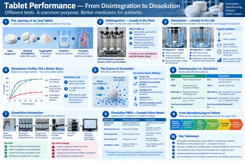
The one idea
Not every load-bearing measurement in a QC lab is a spectrum, a chromatogram, or a mass spectrum. Some read packing instead of bonds (XRPD), a transition instead of a spectrum (DSC/TGA), a cell instead of a molecule (flow cytometry), or a rate instead of a concentration (dissolution) — and each is exactly as rigorous, and exactly as capable of being done sloppily, as the mainline techniques either side of this week.
A diffractogram is a reference-pattern identity test for how a molecule is packed, with a ~5% amorphous-content blind spot that thermal analysis and ssNMR have to cover.
A general single-cell instrument, not just a cell-therapy tool — and a gated result is only as trustworthy as the isotype, FMO, compensation, and calibration controls behind it.
The one routine test about the patient’s experience rather than the molecule’s identity, and a passing result that has never been challenged with a known-defective batch hasn’t earned its trust.
Where the analyst sits
The four sections above share a pattern worth naming: in each, a single trace, pattern, or gated result looks complete on its own and isn’t. A DSC endotherm needs a TGA mass trace to say what it actually is; an XRPD pattern needs to rule out a loading artifact before it says “new form”; a flow-cytometry gate needs its control panel before it says “purity”; a dissolution method needs a deliberately-defective batch before it says “discriminating.” That is the STEAM “A” showing up in four different instruments: knowing what a result can’t tell you until something else confirms it. The refrain: science → evidence → reduced uncertainty → control → regulatory confidence → patient trust.
On the job
These four techniques rarely sit in the same lab group — thermal analysis and XRPD usually live in solid-state/pre-formulation, flow cytometry in a biologics or cell-therapy QC lab, dissolution in routine small-molecule QC. Knowing all four exist, and what each can and can’t answer, matters even if you only ever run one of them.
A polymorph or amorphous-content question almost never gets answered by one of these techniques alone — expect to read a panel (DSC + TGA + XRPD, sometimes PLM or ssNMR) rather than a single number.
Dissolution and Karl Fischer (from last week) are both examples of a test that looks routine and mechanical but is easy to run in a way that quietly invalidates the result — sample handling and method discipline matter as much as the instrument.
For discussion
Of the four techniques this week, which would you expect a job posting to name explicitly, and which would only show up as “or equivalent” in an instrument list? What does that tell you about where each sits in a real lab’s workflow?
A batch fails dissolution with no obvious manufacturing deviation. Sketch an investigation path that uses at least two of this week’s other three techniques before you’d call it a true product failure.
Flow cytometry and dissolution are both described in this week as tests where “the physics is simple but the discipline is hard.” Pick one and explain what “discipline” actually means for it, concretely.
Source note. Each section carries its own source note for the literature and compendial chapters it covers.
1 - Thermal Analysis — DSC and TGA
Differential scanning calorimetry and thermogravimetric analysis: melting, glass transitions and polymorphic transitions by DSC; water, solvent, and decomposition by TGA; and why the two are read together, not separately, before a thermal event is called anything at all.
A one-page overview graphic for this section is still to be produced.
Molecular spectroscopy named this family in passing: the API is the same molecule in every crystal form, and a separate family of techniques reads how it’s packed rather than what bonds it has. Thermal analysis is the simplest member of that family — heat the sample at a controlled rate and watch what happens — and it is usually the first thing run on a new polymorph, salt, or hydrate.
The one idea
DSC and TGA run the same experiment — a controlled temperature ramp — and read two different physical quantities off it: DSC reads heat flow (something absorbing or releasing energy), TGA reads mass. An event that looks identical on a DSC trace alone can mean two completely different things depending on whether TGA shows mass loss at the same temperature — and calling it the wrong one gets a specification wrong.
What each technique reads
Technique
Measures
Typical thermal events
DSC (differential scanning calorimetry)
Heat flow into or out of the sample versus a reference, as a function of temperature
Glass transition (Tg) — a step, not a peak, in an amorphous fraction; melting — a sharp endotherm; polymorphic transition / recrystallization — an exotherm as a metastable form converts; desolvation / dehydration — an endotherm as bound solvent or water leaves
TGA (thermogravimetric analysis)
Sample mass versus temperature
Free water loss (low temperature, gradual); bound/hydrate water or solvent loss (a defined step, often stoichiometric); decomposition (a sharp mass loss, usually well above any pharmaceutically relevant processing temperature)
Reading the pair together
A DSC endotherm at 150 °C could be a true melt, or it could be desolvation — a hydrate or solvate losing bound water or solvent, which also absorbs heat. Run alongside a TGA trace on the same sample: if the DSC endotherm coincides with a mass loss step, it’s desolvation, not melting; if there’s no corresponding mass change, it’s a genuine phase transition. Neither trace alone answers the question — this is the same “orthogonal method” logic as DAD peak purity plus mass balance catching a co-eluting degradant: one measurement’s blind spot is the other’s core signal.
This pairing is also how a hydrate stoichiometry gets confirmed quantitatively — a TGA mass-loss step of, say, 4.5% against a molecular weight lets you calculate whether the sample is a mono-, di-, or hemihydrate, a number a DSC endotherm alone can’t give you.
The amorphous-content connection
An amorphous fraction shows up on DSC as a glass transition — a step in baseline heat flow, not a peak, and it is easy to miss if you aren’t looking for it. This matters because XRPD — the next section — typically can’t see amorphous content below about 5%: DSC (and dynamic vapour sorption) are often what actually catches it, which is why a polymorph or amorphous-content investigation runs both techniques together rather than picking one.
Where the analyst sits
Sample preparation is not incidental to the result: pan type (crimped, hermetic, pinhole) and heating rate both shift the apparent onset temperature of a melt or transition, so a “melting point” reported without its method conditions is not fully specified. A single instrument run is a screening result, not a validated method result — a genuinely unexpected thermal event (an extra endotherm, a shifted Tm) gets confirmed by a second technique before it changes a conclusion about polymorphic form.
On the job
Confirming an incoming lot’s polymorphic form by DSC melting point is a common early task when XRPD access or turnaround is limited — know the reference melting point and its accepted range, not just “does it melt somewhere reasonable.”
A hydrate’s TGA mass-loss step is one of the more reliable numbers in solid-state characterization precisely because it’s stoichiometric — learn to convert a percent mass loss into a hydrate ratio before you’re asked to.
“The DSC looks different from the reference” is a triage problem, not an automatic OOS: check heating rate and pan type against the reference method before treating it as a genuine form change.
For discussion
The same batch run at 5 °C/min and at 20 °C/min gives melting onsets 3 °C apart. Which is “right,” and what does that tell you about reporting a melting point without its method?
A DSC trace shows a single sharp endotherm; TGA on the same sample shows a two-step mass loss ending well before that endotherm. What does that combination imply about the sample’s solid form?
A generic manufacturer’s DSC trace shows a small glass-transition-like step that XRPD doesn’t flag as unusual. Is this worth investigating, and what would you run next?
Source note. Compendial basis: USP ⟨891⟩ (Thermal Analysis), Ph. Eur. 2.2.34 (differential scanning calorimetry), 2.2.35 (thermogravimetry, where adopted). General reference: Giron, Thermal Analysis and Calorimetric Methods in the Characterisation of Polymorphs and Solvates.
2 - X-Ray Powder Diffraction and Crystallography
Reading how a molecule is packed rather than what bonds it has: X-ray powder diffraction as the compendial polymorph/hydrate/salt identity method, single-crystal X-ray for absolute structure, and where polarised light microscopy and solid-state NMR fit around them — plus the amorphous-content blind spot that ties this section back to thermal analysis and dissolution.
A one-page overview graphic for this section is still to be produced.
A molecule’s connectivity — which atoms bond to which — doesn’t change between crystal forms. Its packing does, and packing is exactly what changes a drug’s solubility, dissolution rate, stability, and even its patentability. Thermal analysis infers packing indirectly, from a transition’s energy. X-ray diffraction reads it directly.
The one idea
Every distinct crystal form of a molecule scatters X-rays into its own characteristic pattern, as unique to that packing arrangement as a fingerprint — which makes a diffractogram a reference-pattern identity test, in the same family as the IR and Raman identity checks from molecular spectroscopy, just reading packing instead of bonds.
The technique family
Technique
What it needs
What it gives you
Typical role
X-ray powder diffraction (XRPD)
A bulk powder sample
A diffractogram — peak positions (2θ) and relative intensities unique to the crystal form
The routine compendial method for polymorph, hydrate, and salt-form identity
Single-crystal X-ray diffraction
One suitable single crystal
Absolute molecular structure and packing, unambiguously
Decisive when you can get it, but growing a diffraction-quality crystal is often the limiting step — rare in routine QC
Polarised light microscopy (PLM)
A few particles on a slide
Birefringence — a fast qualitative “is this crystalline, and does it look like the reference”
The cheap first triage before requesting XRPD
Solid-state NMR (ssNMR)
A bulk powder sample
Polymorph identification and quantitation, including amorphous content
The same nucleus-in-a-field physics as the solution NMR sessions earlier in the term, applied to a rigid lattice rather than a tumbling molecule in solution
Why XRPD works
X-rays scatter off the electrons in a crystal’s repeating lattice. Where scattered waves reinforce (Bragg’s law: constructive interference at specific angles set by the lattice spacing), you get a peak; where they cancel, you don’t. Two polymorphs of the same molecule pack their unit cells differently, so their diffractograms — the whole pattern of peak positions — differ, even though every peak in both patterns comes from the identical set of atoms. An identity test compares a sample’s pattern to a reference pattern under a defined acceptance criterion (matching peak positions within a tolerance, not “looks similar”) — the same discipline the course already applied to a UV or IR spectral match.
Preferred orientation is the classic XRPD pitfall: needle- or plate-shaped crystals tend to pack non-randomly on the sample holder, distorting the relative intensities of peaks (though not their positions) — a pattern that looks like a form change on intensity alone can just be a packing artifact from how the powder was loaded.
The amorphous-content blind spot
XRPD’s peaks come from long-range crystalline order; an amorphous fraction has none, and shows up only as a broad, low hump under the crystalline peaks — invisible below roughly 5% amorphous content by routine XRPD. This is the same teaching point flagged in molecular spectroscopy: a small amorphous fraction is more soluble and less stable than the crystalline form, and it’s a classic hidden variable behind a batch that unexpectedly fails dissolution. Below XRPD’s detection limit, DSC’s glass transition, dynamic vapour sorption (extra moisture uptake an amorphous fraction sorbs), and solid-state NMR are what actually catch it — no single technique in this family is complete on its own, which is the same orthogonal-methods lesson the course keeps returning to.
Where the analyst sits
“Matches the reference pattern” needs a stated acceptance criterion before it means anything — which peaks, what 2θ tolerance, and whether intensity is scored at all given preferred orientation. A polymorph-screening report that shows a “new” pattern is a triage problem first: rule out sample-loading artifacts (grind and re-load to randomize orientation) before concluding a genuine new form has appeared.
On the job
PLM is usually the first thing run on an unknown solid — cheap, fast, and it tells you in minutes whether XRPD is even likely to be informative (a fully amorphous sample shows no birefringence at all).
Reading a polymorph-screening report competently means knowing which of several candidate forms is the marketed one and why — usually the most thermodynamically stable form at ambient conditions, defended with the whole technique panel (XRPD, DSC/TGA, PLM), not one trace in isolation.
A “peak intensity looks off” observation is far more often a sample-preparation artifact (preferred orientation, particle size) than a genuine polymorphic change — know to ask about sample loading before escalating.
For discussion
A generic manufacturer’s XRPD pattern matches the reference in peak position but not in relative intensity. Polymorph difference, or artifact? What would you check first, and what would settle it?
Solid-state NMR detects 3% amorphous content that XRPD calls “fully crystalline.” Which result do you trust, and why does the disagreement not mean one technique is wrong?
A batch fails dissolution with no assignable manufacturing deviation. Trace the investigation path through this section and thermal analysis to a plausible root cause.
3 - Flow Cytometry — Instrumentation, Controls, and Reach
Flow cytometry as a general single-cell measurement instrument, not just a cell-therapy tool: fluidics, optics, and the control panel (isotype, FMO, compensation, calibration beads) that make a gating result defensible — plus where the same instrument shows up outside advanced therapies, in viability, apoptosis, and subvisible-particle work.
A one-page overview graphic for this section is still to be produced.
Week 2’s advanced-therapies section introduced flow cytometry as the defining instrument of cell therapy — identity, purity, viability, and transduction efficiency for a CAR-T product. That’s the sharpest application, but it’s not the only one: the same instrument, unmodified, is what a biologics lab reaches for whenever the question is about individual cells or particles, one at a time, rather than a population average.
The one idea
A flow cytometer doesn’t measure a sample — it measures thousands of individual particles per second and reports a distribution. Every number that comes out of it (a percent-positive, a viability figure) is a summary of that distribution, built through a chain of controls and gates that has to be defensible on its own, independent of the biology being measured.
Instrument anatomy
Stage
What it does
What can go wrong
Fluidics
Hydrodynamic focusing forces cells into single file through the interrogation point
Clogging, coincident events (two cells counted as one — a “doublet”)
Optics
Lasers excite fluorophores; dichroic mirrors and bandpass filters route specific wavelengths to detectors
Laser alignment drift, filter degradation, spectral overlap between fluorophores sharing an emission range
Electronics
Photomultiplier tubes (or, in spectral cytometers, avalanche photodiodes) convert light to a voltage pulse; pulse height/area/width are recorded per event
Detector voltage (gain) drift between runs, changing where a population sits on scale run to run
The control panel — what makes a result defensible
A gated percentage is only as trustworthy as the controls that justified where the gates sit:
Control
Purpose
Catches
Unstained control
Establishes autofluorescence baseline
A “positive” that’s really just cellular autofluorescence
Isotype control
A non-specific antibody of the same isotype/fluorophore
Non-specific antibody binding being misread as real marker expression
Fluorescence-minus-one (FMO)
The full panel minus one fluorophore
Where spectral spillover from other channels would place the gate for that one marker
Compensation controls
Single-stained controls for each fluorophore
Sets the compensation matrix (or spectral unmixing) that corrects for overlapping emission spectra
Calibration / CS&T beads
Beads with a certified fluorescence intensity, run before and periodically during acquisition
Instrument drift — laser power, detector gain, alignment — independent of any biological sample
Two analysts can run identical raw data through different gates and report different numbers — Week 2 already made this point for CAR-T purity — and the reason it’s possible at all is that gating logic and order are a method decision, not a downstream analysis step. The control panel above is what constrains that decision to something reproducible between analysts and over time.
Where else this instrument shows up
Outside advanced-therapy identity and potency panels, the same measurement principle answers different pharmaceutical questions:
Viability and apoptosis — Annexin V / 7-AAD or similar dye combinations distinguish live, early-apoptotic, and dead cells, used to monitor a cell line or an in-process cell-therapy intermediate through a hold step or a freeze-thaw.
Microbial enumeration — flow cytometry can count and classify microorganisms directly, an alternative to plate-based methods where a faster result is needed.
Subvisible particle and aggregate counting — a related but distinct family of instruments (flow imaging microscopy) extends the same one-particle-at-a-time logic to counting protein aggregates and subvisible particles, complementing the SEC-MALS/DLS aggregate panel from the biologics CQA table.
Where the analyst sits
A gating scheme is a method, and it needs the same defence a chromatography method needs: why this gate, in this order, bounded by which controls. An instrument calibration record (the CS&T bead trend, not just today’s pass/fail) is often the fastest way to distinguish a genuine biological shift from an instrument that has drifted — check it before re-running the biology.
On the job
Flow cytometry gating is one of the first places a new hire’s independent judgment shows up on a report — expect your gating scheme to be reviewed by someone more senior before your first result goes on a batch record.
Learn to read a compensation matrix and recognise over- or under-compensation (a population that “smears” diagonally on a biaxial plot) before you’re asked to build one.
A viability result that drifts between runs with no change to the biological sample is, more often than not, an instrument-calibration question — check the bead trend before you suspect the cells.
For discussion
Two instruments with different filter sets give different percent-positive results for the same stained sample. How would you demonstrate the two are actually measuring the same thing?
A viability assay run immediately after harvest gives 95%; the same material run four hours later, after a hold step, gives 80%. What would you investigate first — the hold step, the assay, or the instrument?
An analyst tightens a gate slightly and a batch that would have failed a purity specification now passes. What governance should exist around changing a gate after data exists?
Source note. Compendial basis: USP ⟨1027⟩ (Flow Cytometry). General reference: Shapiro, Practical Flow Cytometry (also cited in Week 2’s advanced-therapies section, for the CAR-T application specifically).
4 - Dissolution — The Performance Test
Dissolution as the one routine test about the patient’s experience rather than the molecule’s identity: the USP/Ph. Eur. apparatus, what has to be controlled — medium, sink conditions, agitation — biorelevant versus QC media, discriminating power, IVIVC and biowaivers, and the staged USP ⟨711⟩ acceptance criteria.
Assay tests ask what is in the tablet. Dissolution asks what gets out of it, and how fast — a surrogate for the rate and extent of absorption in a patient. It is the one routine test in this course that is about the patient’s experience rather than the molecule’s identity, and it is where the coating decisions from Week 2’s solid-dosage manufacturing section get proven or disproven.
The one idea
A dissolution method that passes every batch you have ever made is not necessarily good news — it may just mean it isn’t discriminating enough to tell a good batch from a bad one.
The apparatus (USP / Ph. Eur.)
Apparatus
Name
Typical use
1
Basket
Capsules, floating dosage forms
2
Paddle
The default for tablets
3
Reciprocating cylinder
Extended-release, pH-change profiles
4
Flow-through cell
Low-solubility drugs, implants, modified-release; open or closed loop
5–7
Paddle-over-disk, cylinder, reciprocating holder
Transdermals and other special forms
What has to be controlled
The medium (volume, pH, surfactant, degassing), temperature (37 °C), agitation, and — most easily overlooked — sink conditions: enough medium that the dissolved drug never approaches its saturation solubility, or the measured rate is limited by the medium, not by the product. Violate sink conditions and the result describes the bath, not the tablet.
Biorelevant and discriminating media
Simple buffers are used for routine QC; biorelevant media (FaSSIF/FeSSIF, simulating fasted/fed intestinal fluid) are used in development to predict in-vivo behaviour. A good QC method is discriminating — it responds to the formulation and process changes that would matter clinically, and ignores the ones that wouldn’t. Building that discrimination, and then proving it, is the hard part of method development, harder by far than running the test itself.
IVIVC and the biowaiver
An in-vitro / in-vivo correlation links the dissolution profile to a pharmacokinetic profile. A validated Level A IVIVC can support a biowaiver — a formulation or manufacturing-site change approved on dissolution data alone, instead of a new bioequivalence study in humans. This is the direct payoff of a discriminating method: it lets a change be defended with a bench test instead of a clinical one.
Acceptance criteria, staged
USP ⟨711⟩ builds a sampling design directly into the acceptance criteria — not a single pass/fail: test 6 units (S1), and only if that’s inconclusive, 6 more (S2), and only if still inconclusive, 12 more (S3), with the allowed variability widening at each stage. A batch can pass at S1 cleanly, pass at S3 only marginally, or fail outright — and each of those tells you something different about how close to the edge the batch really is.
Where the analyst sits
Is this dissolution method actually discriminating, or does it pass every batch including the ones that would underperform in a patient? That question has no compendial answer — it is answered by deliberately manufacturing batches with known defects (over-compressed, under-coated, wrong particle size) and confirming the method tells them apart. A method that has never been challenged that way hasn’t earned its trust yet, no matter how many batches it has passed.
For discussion
A dissolution method passes every batch you have ever made. How would you go about finding out whether it actually discriminates?
“Sink conditions” — why does violating them make a dissolution result meaningless, and how would you detect that you had?
A batch fails at S1, is retested at S2, and passes comfortably. What does that sequence tell you about the batch that a single S1 result would not?
A functional (extended-release) coating passes appearance and weight-gain checks but the batch fails dissolution — connect this back to Week 2’s coating section: what upstream step would you investigate first?
Source note. Dissolution: USP ⟨711⟩ / ⟨724⟩ / ⟨1092⟩, Ph. Eur. 2.9.3, the FDA dissolution and BCS-biowaiver guidances.